
Posted on 2025/04/19, 3:03 PM By admin22
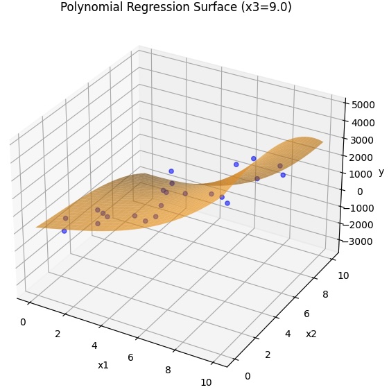
3つの変数から導かれる結果について、多項式回帰モデルを使って見える化をしてみました。
target_functionは対象の任意の関数とします。
|
1 2 3 4 5 6 7 8 9 10 11 12 13 14 15 16 17 18 19 20 21 22 23 24 25 26 27 28 29 30 31 32 33 34 35 36 37 38 39 40 41 42 43 44 45 46 47 48 49 50 51 52 53 54 55 56 57 58 59 60 61 62 63 64 65 66 67 68 69 70 71 72 73 74 75 76 77 78 79 80 81 82 83 84 85 86 87 88 89 90 |
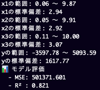
import numpy as np import pandas as pd import matplotlib.pyplot as plt from matplotlib import animation from mpl_toolkits.mplot3d import Axes3D from sklearn.preprocessing import PolynomialFeatures from sklearn.linear_model import LinearRegression from sklearn.metrics import mean_squared_error, r2_score from sklearn.model_selection import train_test_split # --- 任意の非線形関数 --- def target_function(x1, x2, x3): #return 2 * x1**2 - 3 * x2 + 1.5 * x3**2 + 4 * x1 * x3 + np.random.normal(0, 2, size=x1.shape) return 2 * x1**3 - 3 * x2**3 + 1.5 * x3 + 4 * x1 * x3**2 + 2000*np.random.rand(x1.shape[0]) - 1000 # --- データ生成 --- np.random.seed(42) n_samples = 200 x1 = np.random.uniform(0, 10, n_samples) x2 = np.random.uniform(0, 10, n_samples) x3 = np.random.uniform(0, 10, n_samples) y = target_function(x1, x2, x3) df = pd.DataFrame({'x1': x1, 'x2': x2, 'x3': x3, 'y': y}) X = df[['x1', 'x2', 'x3']] y = df['y'] # --- 特徴量変換と学習 --- poly = PolynomialFeatures(degree=3, include_bias=False) X_poly = poly.fit_transform(X) X_train, X_test, y_train, y_test = train_test_split(X_poly, y, test_size=0.2, random_state=42) model = LinearRegression().fit(X_train, y_train) # --- 評価 --- y_pred = model.predict(X_test) mse = mean_squared_error(y_test, y_pred) r2 = r2_score(y_test, y_pred) print(f"x1の範囲: {x1.min():.2f} 〜 {x1.max():.2f}") print(f"x1の標準偏差: {x1.std():.2f}") print(f"x2の範囲: {x2.min():.2f} 〜 {x2.max():.2f}") print(f"x2の標準偏差: {x2.std():.2f}") print(f"x3の範囲: {x3.min():.2f} 〜 {x3.max():.2f}") print(f"x3の標準偏差: {x3.std():.2f}") print(f"yの範囲: {y.min():.2f} 〜 {y.max():.2f}") print(f"yの標準偏差: {y.std():.2f}") print(f"📊 モデル評価") print(f" - MSE: {mse:.3f}") print(f" - R² : {r2:.3f}") # --- 3D アニメーション --- fig = plt.figure(figsize=(10, 7)) ax = fig.add_subplot(111, projection='3d') grid_x1, grid_x2 = np.meshgrid(np.linspace(0, 10, 30), np.linspace(0, 10, 30)) def update(frame): ax.clear() fixed_x3 = frame grid_x3 = np.full_like(grid_x1, fixed_x3) # グリッド点 → DataFrameに変換(列名つけるのが重要) grid_points = np.c_[grid_x1.ravel(), grid_x2.ravel(), grid_x3.ravel()] grid_df = pd.DataFrame(grid_points, columns=['x1', 'x2', 'x3']) # モデル予測 grid_poly = poly.transform(grid_df) grid_y = model.predict(grid_poly).reshape(grid_x1.shape) # 回帰面 ax.plot_surface(grid_x1, grid_x2, grid_y, color='orange', alpha=0.6) # 実データ(x3 ≈ frame) mask = np.isclose(df['x3'], fixed_x3, atol=0.5) ax.scatter(df.loc[mask, 'x1'], df.loc[mask, 'x2'], df.loc[mask, 'y'], color='blue', alpha=0.5) # 軸・表示 ax.set_xlabel('x1') ax.set_ylabel('x2') ax.set_zlabel('y') ax.set_title(f'Polynomial Regression Surface (x3={fixed_x3:.1f})') ax.set_zlim(y.min(), y.max()) ani = animation.FuncAnimation(fig, update, frames=np.linspace(0, 9, 10), interval=1000) plt.show() |
3次元では、2つの変数までしか扱えませんので、x3を固定化しますが、アニメーションによりx3を動かしてみました。
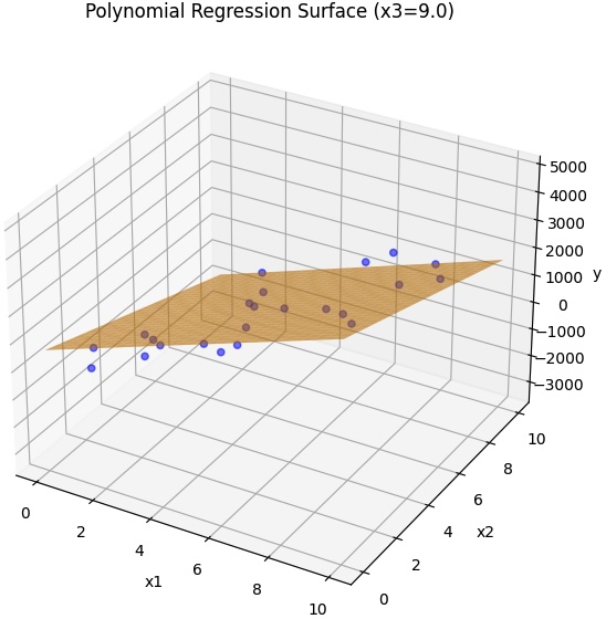
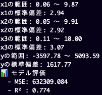
PolynomialFeaturesのdegreeを1にした場合
以上、ChatGPTとの対話から作成しました。
まずシンプルな動作できる形をAIで作っておいて、あとは手作業で作り込んでいくという、こういうコーディングの仕方は、本当に便利です。
Categories: 未分類 タグ: Python